Example-2 of MaxFuse usage between RNA and Protein modality.

In this tutorial, we demonstrate the application of MaxFuse integration and matching across weak-linked modalities. Here we showcase an example between RNA and Protein modality. Specifically, we showcases in this example the matching and integration bewteen: 1. CODEX tonsil iamges with 49 markers (from Kennedy et al. 2021) 2. scRNA-seq tonsil disociated cells (from King et al. 2021)

import numpy as np
import pandas as pd
from scipy.io import mmread

import matplotlib.pyplot as plt
plt.rcParams["figure.figsize"] = (6, 4)

from sklearn.metrics import confusion_matrix, ConfusionMatrixDisplay

import anndata as ad
import scanpy as sc
import maxfuse as mf

import seaborn as sns

/Users/zongming/miniconda3/envs/maxfuse_ipynb/lib/python3.8/site-packages/umap/distances.py:1063: NumbaDeprecationWarning: The 'nopython' keyword argument was not supplied to the 'numba.jit' decorator. The implicit default value for this argument is currently False, but it will be changed to True in Numba 0.59.0. See https://numba.readthedocs.io/en/stable/reference/deprecation.html#deprecation-of-object-mode-fall-back-behaviour-when-using-jit for details.
  @numba.jit()
/Users/zongming/miniconda3/envs/maxfuse_ipynb/lib/python3.8/site-packages/umap/distances.py:1071: NumbaDeprecationWarning: The 'nopython' keyword argument was not supplied to the 'numba.jit' decorator. The implicit default value for this argument is currently False, but it will be changed to True in Numba 0.59.0. See https://numba.readthedocs.io/en/stable/reference/deprecation.html#deprecation-of-object-mode-fall-back-behaviour-when-using-jit for details.
  @numba.jit()
/Users/zongming/miniconda3/envs/maxfuse_ipynb/lib/python3.8/site-packages/umap/distances.py:1086: NumbaDeprecationWarning: The 'nopython' keyword argument was not supplied to the 'numba.jit' decorator. The implicit default value for this argument is currently False, but it will be changed to True in Numba 0.59.0. See https://numba.readthedocs.io/en/stable/reference/deprecation.html#deprecation-of-object-mode-fall-back-behaviour-when-using-jit for details.
  @numba.jit()
/Users/zongming/miniconda3/envs/maxfuse_ipynb/lib/python3.8/site-packages/tqdm/auto.py:21: TqdmWarning: IProgress not found. Please update jupyter and ipywidgets. See https://ipywidgets.readthedocs.io/en/stable/user_install.html
  from .autonotebook import tqdm as notebook_tqdm
/Users/zongming/miniconda3/envs/maxfuse_ipynb/lib/python3.8/site-packages/umap/umap_.py:660: NumbaDeprecationWarning: The 'nopython' keyword argument was not supplied to the 'numba.jit' decorator. The implicit default value for this argument is currently False, but it will be changed to True in Numba 0.59.0. See https://numba.readthedocs.io/en/stable/reference/deprecation.html#deprecation-of-object-mode-fall-back-behaviour-when-using-jit for details.
  @numba.jit()

Data acquire

Since the example data we are uisng in the tutorial excedes the size limit for github repository files, we have uploaded them onto a server and can be easily donwloaded with the code below. Also this code only need to run once for both of the tutorial examples.

import requests, zipfile, io
r = requests.get("http://stat.wharton.upenn.edu/~zongming/maxfuse/data.zip")
z = zipfile.ZipFile(io.BytesIO(r.content))
z.extractall("../")

Data preprocessing

We begin by reading in protein measurements and RNA measurements.

The file format for MaxFuse to read in is adata. The original files we have for RNA was a count table (sparse matrix, row as cells column as rna), and for CODEX it was a csv file with protein expressions (row as cells column as protein). These two files can be turned into adata objects easily.

# read in protein data
protein = pd.read_csv("../data/tonsil/tonsil_codex.csv") # ~178,000 codex cells

We can check how the CODEX data looks like. Note the meta data contained in this csv is not necessary to run MaxFuse. They were used here only for evaluation purpose.

sns.scatterplot(data=protein, x="centroid_x", y="centroid_y", hue = "cluster.term", s = 0.1)

<Axes: xlabel='centroid_x', ylabel='centroid_y'>

# input csv contains meta info, take only protein features
protein_features = ['CD38', 'CD19', 'CD31', 'Vimentin', 'CD22', 'Ki67', 'CD8',
       'CD90', 'CD123', 'CD15', 'CD3', 'CD152', 'CD21', 'cytokeratin', 'CD2',
       'CD66', 'collagen IV', 'CD81', 'HLA-DR', 'CD57', 'CD4', 'CD7', 'CD278',
       'podoplanin', 'CD45RA', 'CD34', 'CD54', 'CD9', 'IGM', 'CD117', 'CD56',
       'CD279', 'CD45', 'CD49f', 'CD5', 'CD16', 'CD63', 'CD11b', 'CD1c',
       'CD40', 'CD274', 'CD27', 'CD104', 'CD273', 'FAPalpha', 'Ecadherin']
# convert to AnnData
protein_adata = ad.AnnData(
    protein[protein_features].to_numpy(), dtype=np.float32
)
protein_adata.var_names = protein[protein_features].columns

Then we read in the RNA files and convert to adata format too.

# read in RNA data
rna = mmread("../data/tonsil/tonsil_rna_counts.txt") # rna count as sparse matrix, 10k cells (RNA)
rna_names = pd.read_csv('../data/tonsil/tonsil_rna_names.csv')['names'].to_numpy()
# convert to AnnData
rna_adata = ad.AnnData(
    rna.tocsr(), dtype=np.float32
)
rna_adata.var_names = rna_names

Optional: meta data for the cells. In this case we are using them to evaluate the integration results, but for actual running, MaxFuse does not require you have this information.

# read in celltyle labels
metadata_rna = pd.read_csv('../data/tonsil/tonsil_rna_meta.csv')
labels_rna = metadata_rna['cluster.info'].to_numpy()
labels_codex = protein['cluster.term'].to_numpy()

protein_adata.obs['celltype'] = labels_codex
rna_adata.obs['celltype'] = labels_rna

Here we are integrating protein and RNA data, and most of the time there are name differences between protein (antibody) and their corresponding gene names.

These “weak linked” features will be used during initialization (we construct two arrays, rna_shared and protein_shared, whose columns are matched, and the two arrays can be used to obtain the initial matching).

To construct the feature correspondence in straight forward way, we prepared a .csv file containing most of the antibody name (seen in cite-seq or codex antibody names etc) and their corresponding gene names:

correspondence = pd.read_csv('../data/protein_gene_conversion.csv')
correspondence.head()

	Protein name	RNA name
0	CD80	CD80
1	CD86	CD86
2	CD274	CD274
3	CD273	PDCD1LG2
4	CD275	ICOSLG

But of course this files does contain all names including custom names in new assays. If a certain correspondence is not found, either it is missing in the other modality, or you should customly add the name conversion to this .csv file.

rna_protein_correspondence = []

for i in range(correspondence.shape[0]):
    curr_protein_name, curr_rna_names = correspondence.iloc[i]
    if curr_protein_name not in protein_adata.var_names:
        continue
    if curr_rna_names.find('Ignore') != -1: # some correspondence ignored eg. protein isoform to one gene
        continue
    curr_rna_names = curr_rna_names.split('/') # eg. one protein to multiple genes
    for r in curr_rna_names:
        if r in rna_adata.var_names:
            rna_protein_correspondence.append([r, curr_protein_name])

rna_protein_correspondence = np.array(rna_protein_correspondence)

# Columns rna_shared and protein_shared are matched.
# One may encounter "Variable names are not unique" warning,
# this is fine and is because one RNA may encode multiple proteins and vice versa.
rna_shared = rna_adata[:, rna_protein_correspondence[:, 0]].copy()
protein_shared = protein_adata[:, rna_protein_correspondence[:, 1]].copy()

/Users/zongming/miniconda3/envs/maxfuse_ipynb/lib/python3.8/site-packages/anndata/_core/anndata.py:1832: UserWarning: Variable names are not unique. To make them unique, call `.var_names_make_unique`.
  utils.warn_names_duplicates("var")
/Users/zongming/miniconda3/envs/maxfuse_ipynb/lib/python3.8/site-packages/anndata/_core/anndata.py:1832: UserWarning: Variable names are not unique. To make them unique, call `.var_names_make_unique`.
  utils.warn_names_duplicates("var")

Then we retrieve the shared features. Normally we should not use all the shared featues, as some of the shared feature RNA are not very variable, and inputing low quality features could potentially decrease the performance of MaxFuse. In this case we only use RNA or Protein features that are variable (larger than a certain threshold).

# Make sure no column is static
mask = (
    (rna_shared.X.toarray().std(axis=0) > 0.5)
    & (protein_shared.X.std(axis=0) > 0.1)
)
rna_shared = rna_shared[:, mask].copy()
protein_shared = protein_shared[:, mask].copy()
print([rna_shared.shape,protein_shared.shape])

[(12977, 32), (178919, 32)]

We apply standard Scanpy preprocessing steps to rna_shared. We skipped the processing steps for protein_shared because the input CODEX data was already normalized et.

# process rna_shared
sc.pp.normalize_total(rna_shared)
sc.pp.log1p(rna_shared)
sc.pp.scale(rna_shared)

/Users/zongming/miniconda3/envs/maxfuse_ipynb/lib/python3.8/site-packages/scanpy/preprocessing/_normalization.py:197: UserWarning: Some cells have zero counts
  warn(UserWarning('Some cells have zero counts'))

# plot UMAP of rna cells based only on rna markers with protein correspondence

sc.pp.neighbors(rna_shared, n_neighbors=15)
sc.tl.umap(rna_shared)
sc.pl.umap(rna_shared, color='celltype')

/Users/zongming/miniconda3/envs/maxfuse_ipynb/lib/python3.8/site-packages/scanpy/plotting/_tools/scatterplots.py:392: UserWarning: No data for colormapping provided via 'c'. Parameters 'cmap' will be ignored
  cax = scatter(

# plot UMAPs of codex cells based only on protein markers with rna correspondence
# due to a large number of codex cells, this can take a while. uncomment below to plot.

# sc.pp.neighbors(protein_shared, n_neighbors=15)
# sc.tl.umap(protein_shared)
# sc.pl.umap(protein_shared, color='celltype')

rna_shared = rna_shared.X.copy()
protein_shared = protein_shared.X.copy()

We again apply standard Scanpy preprocessing steps to all available RNA measurements and protein measurements (not just the shared ones) to get two arrays, rna_active and protein_active, which are used for iterative refinement. Again if the input data is already processed, these steps can be skipped.

# process all RNA features
sc.pp.normalize_total(rna_adata)
sc.pp.log1p(rna_adata)
sc.pp.highly_variable_genes(rna_adata, n_top_genes=5000)
# only retain highly variable genes
rna_adata = rna_adata[:, rna_adata.var.highly_variable].copy()
sc.pp.scale(rna_adata)

# plot UMAPs of rna cells based on all active rna markers

sc.pp.neighbors(rna_adata, n_neighbors=15)
sc.tl.umap(rna_adata)
sc.pl.umap(rna_adata, color='celltype')

WARNING: You’re trying to run this on 5000 dimensions of `.X`, if you really want this, set `use_rep='X'`.
         Falling back to preprocessing with `sc.pp.pca` and default params.

/Users/zongming/miniconda3/envs/maxfuse_ipynb/lib/python3.8/site-packages/scanpy/plotting/_tools/scatterplots.py:392: UserWarning: No data for colormapping provided via 'c'. Parameters 'cmap' will be ignored
  cax = scatter(

# plot UMAPs of protein cells based on all active protein markers
# due to a large number of codex cells, this can take a while. uncomment below to plot.

# sc.pp.neighbors(protein_adata, n_neighbors=15)
# sc.tl.umap(protein_adata)
# sc.pl.umap(protein_adata, color='celltype')

# make sure no feature is static
rna_active = rna_adata.X
protein_active = protein_adata.X
rna_active = rna_active[:, rna_active.std(axis=0) > 1e-5] # these are fine since already using variable features
protein_active = protein_active[:, protein_active.std(axis=0) > 1e-5] # protein are generally variable

# inspect shape of the four matrices
print(rna_active.shape)
print(protein_active.shape)
print(rna_shared.shape)
print(protein_shared.shape)

(12977, 5000)
(178919, 46)
(12977, 32)
(178919, 32)

Fitting MaxFuse

Step I: preparations

We now have four arrays. rna_shared and protein_shared are used for finding initial pivots, whereas rna_active and protein_active are used for iterative refinement.

The main object for running MaxFuse pipeline is mf.model.Fusor, and its constructor takes the above four arrays as input.

If your data have not been clustered and annotated, you can leave labels1 and labels2 to be None, then MaxFuse will automatically run clustering algorithms to fill them in.

Optional: If your data have already been clustered (and you trust your annotation is optimal and should be used to guide the MaxFuse smoothing steps), you could supply them as numpy arrays to labels1 and labels2.

# call constructor for Fusor object
# which is the main object for running MaxFuse pipeline
fusor = mf.model.Fusor(
    shared_arr1=rna_shared,
    shared_arr2=protein_shared,
    active_arr1=rna_active,
    active_arr2=protein_active,
    labels1=None,
    labels2=None
)

To reduce computational complexity, we call split_into_batches to fit the batched version of MaxFuse.

Internally, MaxFuse will solve a few linear assignment problems of size \(n_1 \times n_2\), where \(n_1\) and \(n_2\) (with \(n_1\leq n_2\) by convention) are the sample sizes of the two modalities (after batching and metacell construction). max_outward_size specifis the maximum value of \(n_1\).

matching_ratio specifies approximately the ratio of \(n_2/n_1\). The larger it is, the more candidate cells in the second modality MaxFuse will seek for to match each cell/metacell in the first modality.

metacell_size specifies the average size of the metacells in the first modality.

Since this integration process is larger (more CODEX cells), we could increase the max_outward_size as long as the memory can accomodate that.

fusor.split_into_batches(
    max_outward_size=8000,
    matching_ratio=4,
    metacell_size=2,
    verbose=True
)

The first data is split into 1 batches, average batch size is 12977, and max batch size is 12977.
The second data is split into 5 batches, average batch size is 35783, and max batch size is 35787.
Batch to batch correspondence is:
  ['0<->0', '0<->1', '0<->2', '0<->3', '0<->4'].

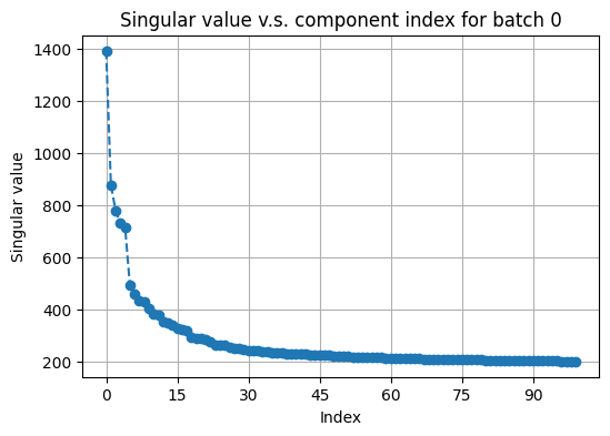
The next step is to construct appropriate nearest-neighbor graphs for each modality with all features available. But before that, we plot the singular values of the two active arrays to determine how many principal components (PCs) to keep when doing graph construction.

# plot top singular values of avtive_arr1 on a random batch
fusor.plot_singular_values(
    target='active_arr1',
    n_components=None # can also explicitly specify the number of components
)

(<Figure size 600x400 with 1 Axes>,
 <Axes: title={'center': 'Singular value v.s. component index for batch 0'}, xlabel='Index', ylabel='Singular value'>)

# plot top singular values of avtive_arr2 on a random batch
fusor.plot_singular_values(
    target='active_arr2',
    n_components=None
)

(<Figure size 600x400 with 1 Axes>,
 <Axes: title={'center': 'Singular value v.s. component index for batch 4'}, xlabel='Index', ylabel='Singular value'>)

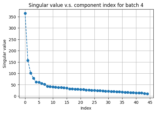
Inspecting the “elbows”, we choose the number of PCs to be 40 for both RNA and 15 for protein active data. We then call construct_graphs to compute nearest-neighbor graphs as needed.

fusor.construct_graphs(
    n_neighbors1=15,
    n_neighbors2=15,
    svd_components1=40,
    svd_components2=15,
    resolution1=2,
    resolution2=2,
    # if two resolutions differ less than resolution_tol
    # then we do not distinguish between then
    resolution_tol=0.1,
    verbose=True
)

Aggregating cells in arr1 into metacells of average size 2...
Constructing neighborhood graphs for cells in arr1...
Now at batch 0...
Graph construction finished!
Clustering into metacells...
Now at batch 0...
Metacell clustering finished!
Constructing neighborhood graphs for cells in arr1...
Now at batch 0...
Graph construction finished!
Clustering the graphs for cells in arr1...
Now at batch 0...
Graph clustering finished!
Constructing neighborhood graphs for cells in arr2...
Now at batch 0...
Now at batch 1...
Now at batch 2...
Now at batch 3...
Now at batch 4...
Graph construction finished!
Clustering the graphs for cells in arr2...
Now at batch 0...
Now at batch 1...
Now at batch 2...
Now at batch 3...
Now at batch 4...
Graph clustering finished!

Step II: finding initial pivots

We then use shared arrays whose columns are matched to find initial pivots. Before we do so, we plot top singular values of two shared arrays to determine how many PCs to use.

# plot top singular values of shared_arr1 on a random batch
fusor.plot_singular_values(
    target='shared_arr1',
    n_components=None,
)

(<Figure size 600x400 with 1 Axes>,
 <Axes: title={'center': 'Singular value v.s. component index for batch 0'}, xlabel='Index', ylabel='Singular value'>)

# plot top singular values of shared_arr2 on a random batch
fusor.plot_singular_values(
    target='shared_arr2',
    n_components=None
)

(<Figure size 600x400 with 1 Axes>,
 <Axes: title={'center': 'Singular value v.s. component index for batch 3'}, xlabel='Index', ylabel='Singular value'>)

We choose to use 25 PCs for rna_shared and 20 PCs for protein_shared.

We then call find_initial_pivots to compute initial set of matched pairs. In this function, wt1 (resp. wt2) is a number between zero and one that specifies the weight on the smoothing target for the first (resp. second) modality. The smaller it is, the greater the strength of fuzzy smoothing. When the weight is one, then there is no smoothing at all, meaning the original data will be used.

Previously in the cite-seq example we used wt1 = 0.7 and wt2 = 0.7. In the case of integration that involves spatial data, we encourage using wt1 = 0.3 and wt2 = 0.3 since such datasets are usually “weaker” in linkage and requires stronger “smoothing”.

fusor.find_initial_pivots(
    wt1=0.3, wt2=0.3,
    svd_components1=25, svd_components2=20
)

Now at batch 0<->0...
Now at batch 0<->1...
Now at batch 0<->2...
Now at batch 0<->3...
Now at batch 0<->4...
Done!

Now, we have a set of initial pivots that store the matched pairs when only the information in the shared arrays is used. The information on initial pivots are stored in the internal field fusor._init_matching that is invisible to users.

Step III: finding refined pivots

We now use the information in active arrays to iteratively refine initial pivots. We plot the top canonical correlations to choose the best number of components in canonical correlation analysis (CCA).

# plot top canonical correlations in a random batch
fusor.plot_canonical_correlations(
    svd_components1=50,
    svd_components2=None,
    cca_components=45
)

(<Figure size 600x400 with 1 Axes>,
 <Axes: title={'center': 'Canonical correlation v.s. component index for batch 0<->3'}, xlabel='Index', ylabel='Canonical correlation'>)

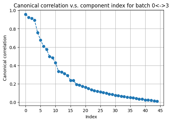
A quick check on the previous plot gives a rough guide on what the refine_pivots parameters should be picked.

Note: here that the n_iters number we choosed 1, as in low snr datasets (eg. Spatial-omis) increase amount of iteration might degrade the performance.

fusor.refine_pivots(
    wt1=0.3, wt2=0.3,
    svd_components1=40, svd_components2=None,
    cca_components=25,
    n_iters=1,
    randomized_svd=False,
    svd_runs=1,
    verbose=True
)

Now at batch 0<->0...
Now at batch 0<->1...
Now at batch 0<->2...
Now at batch 0<->3...
Now at batch 0<->4...
Done!

Note: here we can see filter_prop we increased the pivot filtering to 0.5 compared to previous example. We found harsher filtering for integrations that involves spatial-omics is more beneficial.

fusor.filter_bad_matches(target='pivot', filter_prop=0.5)

Begin filtering...
Now at batch 0<->0...
Now at batch 0<->1...
Now at batch 0<->2...
Now at batch 0<->3...
Now at batch 0<->4...
16190/32380 pairs of matched cells remain after the filtering.
Fitting CCA on pivots...
Scoring matched pairs...
8885/12977 cells in arr1 are selected as pivots.
16190/178919 cells in arr2 are selected as pivots.
Done!

Optional: quick check the performance based on cell type accuracy (pivot matching).

pivot_matching = fusor.get_matching(order=(2, 1),target='pivot')

lv1_acc = mf.metrics.get_matching_acc(matching=pivot_matching,
    labels1=labels_rna,
    labels2=labels_codex,
    order = (2,1)
)
lv1_acc

0.9553428042001235

# We can inspect the first pivot pair.
[pivot_matching[0][0], pivot_matching[1][0], pivot_matching[2][0]]

[3249, 13, 0.8213132906237305]

cm = confusion_matrix(labels_rna[pivot_matching[0]], labels_codex[pivot_matching[1]])
ConfusionMatrixDisplay(
    confusion_matrix=np.round((cm.T/np.sum(cm, axis=1)).T*100),
    display_labels=np.unique(labels_rna)
).plot()

<sklearn.metrics._plot.confusion_matrix.ConfusionMatrixDisplay at 0x1746d8640>

Note: Since we have the refine_pivots now, we can theoratically co-embedding the full dataset into CCA space (as described in tutorial-1). However, in the case that invovles low-snr datasets (eg. spatial-omics), we do not suggest projecting all the cells into a common space without any filtering steps. We will describe this process after the propogation step.

Step IV: propagation

Refined pivots can only give us a pivot matching that captures a subset of cells. In order to get a full matching that involves all cells during input, we need to call propagate.

fusor.propagate(
    svd_components1=40,
    svd_components2=None,
    wt1=0.7,
    wt2=0.7,
)

Now at batch 0<->0...
Now at batch 0<->1...
Now at batch 0<->2...
Now at batch 0<->3...
Now at batch 0<->4...
Done!

We call filter_bad_matches with target=propagated to optionally filter away a few matched pairs from propagation.

Note: In the best scenario, we would prefer all cells in the full dataset can be matched accross modality. However, in the case that invovles low-snr datasets (eg. spatial-omics), many cells are noisy (or lack of information) and should not be included in downstream cross-modality analysis. We suggest in such scenarios, filter_prop should be set around 0.1-0.4.

fusor.filter_bad_matches(
    target='propagated',
    filter_prop=0.3
)

Begin filtering...
Now at batch 0<->0...
Now at batch 0<->1...
Now at batch 0<->2...
Now at batch 0<->3...
Now at batch 0<->4...
125243/178919 pairs of matched cells remain after the filtering.
Scoring matched pairs...
Done!

We use get_matching with target='full_data' to extract the full matching.

Because of the batching operation, the resulting matching may contain duplicates. The order argument determines how those duplicates are dealt with. order=None means doing nothing and returning the matching with potential duplicates; order=(1, 2) means returning a matching where each cell in the first modality contains at least one match in the second modality; order=(2, 1) means returning a matching where each cell in the second modality contains at least one match in the first modality.

Note: Since we filtered out some cell pairs here, not all cells in the full dataset has matches.

full_matching = fusor.get_matching(order=(2, 1), target='full_data')

Since we are doing order=(2, 1) here, the matching info is all the cells (10k) in mod 2 (protein) has at least one match cell in the RNA modality. Note that the matched cell in RNA could be duplicated, as protein cells could be matched to the same RNA cell. For a quick check on matching format:

pd.DataFrame(list(zip(full_matching[0], full_matching[1], full_matching[2])),
             columns = ['mod1_indx', 'mod2_indx', 'score'])
# columns: cell idx in mod1, cell idx in mod2, and matching scores

	mod1_indx	mod2_indx	score
0	3249	13	0.821313
1	4694	26	0.716275
2	8707	45	0.899197
3	5677	57	0.641894
4	12159	62	0.848711
...	...	...	...
141428	5069	178911	0.340677
141429	3084	178913	0.179931
141430	10842	178916	0.268173
141431	3201	178917	0.651751
141432	6183	178918	0.744751

141433 rows × 3 columns

# compute the cell type level matching accuracy, for the full (filtered version) dataset
lv1_acc = mf.metrics.get_matching_acc(matching=full_matching,
    labels1=labels_rna,
    labels2=labels_codex
)
lv1_acc

0.9108835985943875

Step V: downstream analysis

As mentioned before, we want to draw a UMAP in the joint-embedding space, but for the filtered version of cells. For the low-snr datasets (eg. spatial-omics), we suggest only using cells that survived the propogation filtering step.

rna_cca, protein_cca_sub = fusor.get_embedding(
    active_arr1=fusor.active_arr1,
    active_arr2=fusor.active_arr2[full_matching[1],:] # cells in codex remained after filtering
)

Since we have ~170,000 cells for CODEX, calculating UMAP for the full dataset will take a while, for showcasing we can just subsample a smaller sample.

np.random.seed(42)
subs = 13000
randix = np.random.choice(protein_cca_sub.shape[0],subs, replace = False)

dim_use = 15 # dimensions of the CCA embedding to be used for UMAP etc

cca_adata = ad.AnnData(
    np.concatenate((rna_cca[:,:dim_use], protein_cca_sub[randix,:dim_use]), axis=0),
    dtype=np.float32
)
cca_adata.obs['data_type'] = ['rna'] * rna_cca.shape[0] + ['protein'] * subs
cca_adata.obs['cell_type'] = list(np.concatenate((labels_rna,
                                                  labels_codex[full_matching[1]][randix]), axis = 0))

sc.pp.neighbors(cca_adata, n_neighbors=15)
sc.tl.umap(cca_adata)
sc.pl.umap(cca_adata, color='data_type')

/Users/zongming/miniconda3/envs/maxfuse_ipynb/lib/python3.8/site-packages/scanpy/plotting/_tools/scatterplots.py:392: UserWarning: No data for colormapping provided via 'c'. Parameters 'cmap' will be ignored
  cax = scatter(

sc.pl.umap(cca_adata, color='cell_type')

/Users/zongming/miniconda3/envs/maxfuse_ipynb/lib/python3.8/site-packages/scanpy/plotting/_tools/scatterplots.py:392: UserWarning: No data for colormapping provided via 'c'. Parameters 'cmap' will be ignored
  cax = scatter(

Step VI: more custom analysis

There could be potentially more custom analysis produced by MaxFuse.

For example in our manuscript, we looked at the distribution or RNA counts on a CODEX tissue. Such information can be directly retrieved from the full_matching table we produced previously (eg. transfer the RNA information onto CODEX for each matched single cell pair).

Moreover, analysis like label transfer can also be implemented, either by directly transfering the labels across matched pairs, or run a KNN process on the joint-embedding that MaxFuse produced, and do majority voting, or some kind of weighted decision based on the distance scores from MaxFuse.

Since these type of analysis are highly customized, we did not implment them in the MaxFuse pipeline. However, please give us feedbacks on whether a specific type of task should be included.